Resolution

Code status: The code on this page was corrected on 17 September 2026 against the current Earth Engine Data Catalog and API documentation. It has not been executed against Earth Engine. Screenshots, printed values and described outputs come from earlier versions of this lesson and may differ from what the corrected code produces.

In this tutorial, we will cover the four different types of resolution by looking at some of the most well-known satellite platforms. At the completion of this tutorial, you will understand how to select the appropriate data for your use case, visualize the data, and begin to extract insights from it.

We will focus on the four primary types of resolution:

1. Spatial
2. Temporal
3. Radiometric
4. Spectral

While doing this, we will introduce three of the most well-known satellite missions:

1. MODIS
2. Landsat
3. Sentinel

Spatial Resolution

Spatial resolution refers to the real-world representation of each pixel. This ranges widely, with the private satellite company Maxar announcing 15cm resolution, Sentinel at 10m, Landsat at 30m, and MODIS at 500m. There are also large global products that have spatial resolution in the kilometers. The key point in dealing with spatial resolution is ensuring that your analysis drives your data collection, as there are tradeoffs involved. Using high-resolution imagery can be expensive, both monetarily and computationally, if conducting continent-wide analysis. Yet using low-resolution imagery will not be effective if your use case necessitates identifying individual buildings or small vehicles. Understanding the appropriate spatial resolution needed for your analysis is essential, and is why there are different platforms that focus on different spatial resolutions.

In practice, spatial resolution depends on the projection of the sensor’s instantaneous field of view (IFOV) of the ground and how a set of radiometric measurements are resampled into a regular grid. To see the difference in spatial resolution resulting from different sensors, let’s visualize data from the three primary platforms.

MODIS

There are two Moderate Resolution Imaging Spectroradiometers ( MODIS) aboard the Terra and Aqua satellites. Different MODIS bands produce data at different spatial resolutions: 250m for the red and near-infrared bands, 500m for the shortwave infrared bands, and 1km for the thermal infrared bands. Data from the MODIS platforms are used to produce a large number of data sets having daily, weekly, 16-day, monthly, and annual time steps. You can find current MODIS datasets available in Earth Engine in the MODIS catalog.

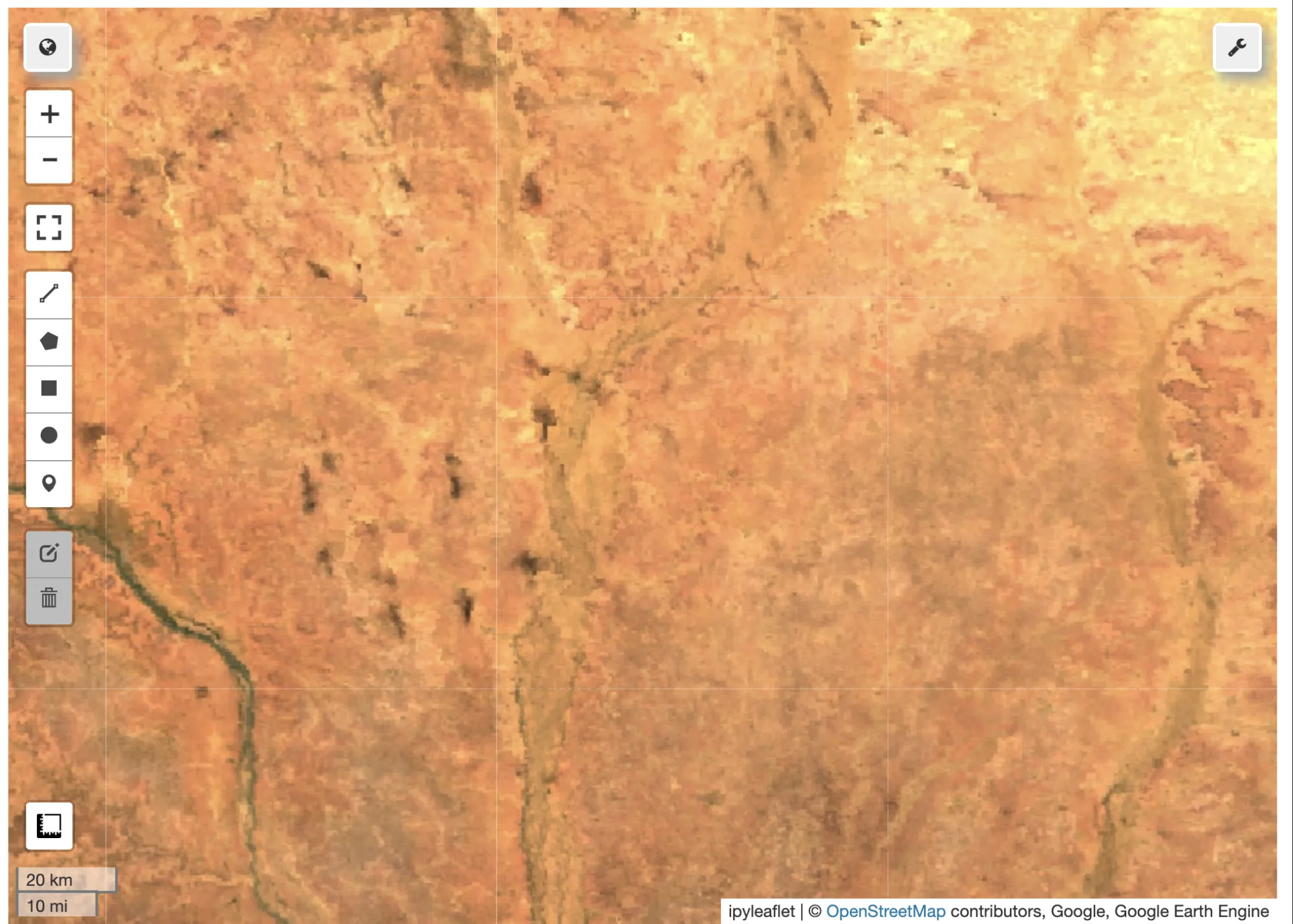
In the code below, we are working with the MODIS Terra Surface Reflectance 8-day Global 500m resolution data. Change the number in the zoom variable to scroll in and out - notice that when scrolled in, each pixel is quite large and granular.

Python setup: every Python cell on this page assumes this block has already run in the same session. Registering a Cloud project and authenticating are covered in Getting Started with Earth Engine.

import ee
import geemap

ee.Authenticate()  # opens the sign-in flow when no stored credentials exist
ee.Initialize(project='your-cloud-project-id')  # use your registered Cloud project ID

def build_map(lat, lon, zoom, vis_params, image, name):
    m = geemap.Map(center=[lat, lon], zoom=zoom)
    m.addLayer(image, vis_params, name)
    return m

var lat = 13.7; var lon = 2.54; var zoom = 10
var image = ee.ImageCollection('MODIS/061/MOD09A1')
                  .filter(ee.Filter.date('2018-01-01', '2018-05-01'))
                  .first();
var bands = ['sur_refl_b01', 'sur_refl_b04', 'sur_refl_b03']
var vizParams = {
  bands: bands,
  min: -100.0,
  max: 3000.0,
};
// Center the map on the study area in Niger
Map.setCenter(lon, lat, zoom);
Map.addLayer(image, vizParams, 'True Color');

lat = 13.7; lon = 2.54
zoom = 10
image_collection_name = 'MODIS/061/MOD09A1'
date_start = '2018-01-01'
date_end = '2018-05-01'
name = 'True Color'
image = (ee.ImageCollection(image_collection_name)
         .filter(ee.Filter.date(date_start, date_end))
         .first())
bands = ['sur_refl_b01', 'sur_refl_b04', 'sur_refl_b03']
vizParams = {
    'bands': bands, 
    'min': -100,
    'max': 3000
}
map = build_map(lat, lon, zoom, vizParams, image, name)
map

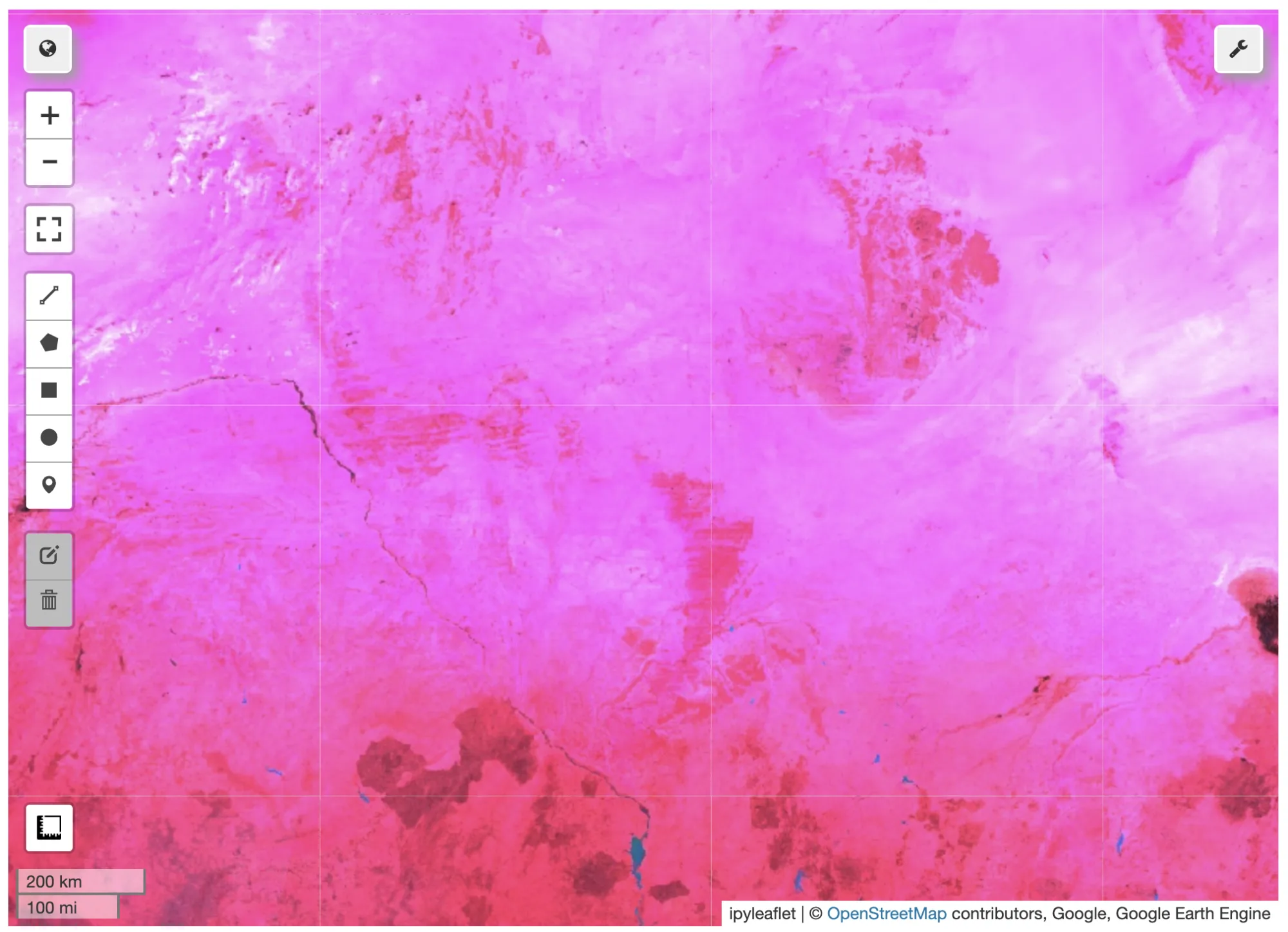
We will discuss some of the benefits of working with false-color imagery in later sections, but we can modify the bands we want to visualize. In this case, we are using a random set of bands, where the value of band six is visualized with red, band three is visualized with green, and band one with blue. Because the value of band six has a higher range, this image shows up with a heavy red presence.

var lat = 13.7; var lon = 2.54; var zoom = 10
var dataset = ee.ImageCollection('MODIS/061/MOD09A1')
                  .filter(ee.Filter.date('2018-01-01', '2018-05-01'))
                  .first();
var bands = ['sur_refl_b06', 'sur_refl_b03', 'sur_refl_b01'];
var modisVis = {
  bands: bands, 
  min: 0, 
  max: 3000
};
var zoom = 10
Map.setCenter(lon, lat, zoom);
Map.addLayer(dataset, modisVis, 'MODIS');

# Define the variables
lat = 13.7; lon = 2.54; zoom = 10
image = (
    ee.ImageCollection('MODIS/061/MOD09A1')
         .filterDate('2018-01-01', '2018-05-01')
         .first())
bands = ['sur_refl_b06', 'sur_refl_b03', 'sur_refl_b01']
vizParams = {
    'bands': bands, 
    'min': 0, 
    'max': 3000
}
map = build_map(lat, lon, zoom, vizParams, image, 'MODIS')
map

Compare the size of MODIS pixels to objects on the ground. It may help to turn on the satellite basemap and lower the opacity of the layer (top right of the map section of the code editor) to see high-resolution data for comparison.

Print the size of the pixels (in meters) to the console. You can read more about how Google Earth Engine works with scale in their documentation. The catalog lists a 500 m pixel size for these bands, but that is the product’s nominal label. MOD09A1 is distributed on the MODIS Sinusoidal grid (see the projections guide), whose “500 m” cells are about 463 m wide (each 10° MODIS tile, about 1,112 km across at the equator, is divided into 2,400 cells), so nominalScale() is expected to report a value near 463 m rather than a round 500. The value describes the grid cell size of the data; it has nothing to do with how the map tiles are drawn.

var dataset = ee.ImageCollection('MODIS/061/MOD09A1')
                  .filter(ee.Filter.date('2018-01-01', '2018-05-01'))
                  .first();
// Get the scale of the data from the first band's projection:
var modisScale = dataset.select('sur_refl_b01')
    .projection()
    .nominalScale();
print('MODIS scale:', modisScale);

dataset = (ee.ImageCollection('MODIS/061/MOD09A1')
           .filter(ee.Filter.date('2018-01-01', '2018-05-01'))
           .first());
# Get the scale of the data from the first band's projection:
modisScale = (dataset.select('sur_refl_b01')
    .projection()
    .nominalScale());
print('MODIS scale:', modisScale.getInfo());

Question 1: What is the size of the pixel?

Landsat

Multi-spectral scanners (MSS) were flown aboard Landsat missions 1-5 and have a spatial resolution of 60 meters. Let’s look at the USGS Landsat 5 MSS Collection 2 Tier 1 Raw Scenes. We can find the information about the bands for Landsat 5 MSS in the documentation and then build out some imagery. MSS has four bands: B1 (green), B2 (red), B3 (near infrared 1) and B4 (near infrared 2).

Note: always refer to the documentation to make sure you are working with the correct information. The same band name can mean different things in different collections: B4 is the second near-infrared band for Landsat 5 MSS and the near-infrared band for Landsat 5 TM, but the red band for Landsat 8.

var lat = 37.22; var lon = -80.42; var zoom = 12
// Landsat 5 MSS Collection 2 Tier 1 raw scenes (digital numbers)
var image = ee.ImageCollection('LANDSAT/LM05/C02/T1')
                  .filterBounds(ee.Geometry.Point(lon, lat))
                  .filterDate('1985-01-01', '1989-12-31');
// Near infrared 1, red and green
var bands = ['B3', 'B2', 'B1']
var vizParams = {
    'bands': bands, 
    'min': 0,
    'max': 150
}
Map.setCenter(lon, lat, zoom);
Map.addLayer(image, vizParams, 'Landsat 5 MSS');

lat = 37.22; lon = -80.42; zoom = 12
# Landsat 5 MSS Collection 2 Tier 1 raw scenes (digital numbers)
image = (ee.ImageCollection('LANDSAT/LM05/C02/T1')
                  .filterBounds(ee.Geometry.Point(lon, lat))
                  .filterDate('1985-01-01', '1989-12-31'));
# Near infrared 1, red and green
bands = ['B3', 'B2', 'B1']
vizParams = {
    'bands': bands, 
    'min': 0,
    'max': 150
}
map = build_map(lat, lon, zoom, vizParams, image, 'Landsat 5 MSS')
map

As before, let’s extract the nominal scale from the first image’s B1 band and print it to the console. The catalog lists a 60 m pixel size for B1, B2 and B3, so that is the value to expect.

var mssScale = image.first().select('B1').projection().nominalScale();
print('MSS scale:', mssScale);

mssScale = image.first().select('B1').projection().nominalScale();
print('MSS scale:', mssScale.getInfo());

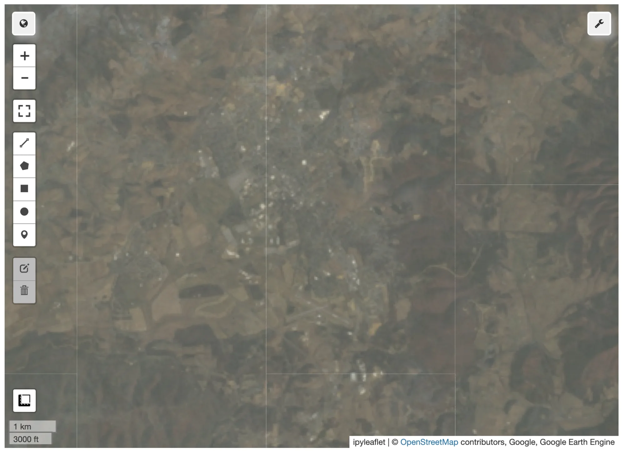
The Thematic Mapper (TM) was flown aboard Landsat 4-5 and then succeeded by the Enhanced Thematic Mapper (ETM+) aboard Landsat 7 and the Operational Land Imager (OLI) / Thermal Infrared Sensor (TIRS) sensors aboard Landsat 8. TM data have a spatial resolution of 30 meters, which has remained the Landsat standard resolution. We can check this by importing the ‘USGS Landsat 5 TM Collection 2 Tier 1 TOA Reflectance’ and visualizing it; its catalog page lists a 30 m pixel size for every band, and you can print the scale the same way as for MSS. For some additional discussion about Landsat 5, see the USGS Landsat 5 mission page.

You can find the information on the different Landsat missions on the GEE datasets page. There is some fascinating information about the history of the Landsat missions, but for the purposes of this exercise, find the Landsat mission that you are interested in and navigate to the ‘Bands’ tab - here you can find the naming for the bands and the associated description.

var lat = 37.22; var lon = -80.42; var zoom = 12
var image = ee.ImageCollection("LANDSAT/LT05/C02/T1_TOA")
  .filterDate('2011-01-01', '2011-12-31');
var bands = ['B4', 'B3', 'B2'];
var vizParams = {
  bands: bands,
  min: 0.0,
  max: 0.4,
  gamma: 1.2,
};
Map.setCenter(lon, lat, zoom);
Map.addLayer(image, vizParams, 'False Color (432)');

lat = 37.22; lon = -80.42; zoom = 12
image = (ee.ImageCollection("LANDSAT/LT05/C02/T1_TOA")
  .filterDate('2011-01-01', '2011-12-31'));
bands = ['B4', 'B3', 'B2'];
vizParams = {
  'bands': bands,
  'min': 0.0,
  'max': 0.4,
  'gamma': 1.2,
};
map = build_map(lat, lon, zoom, vizParams, image, 'False Color (432)')
map

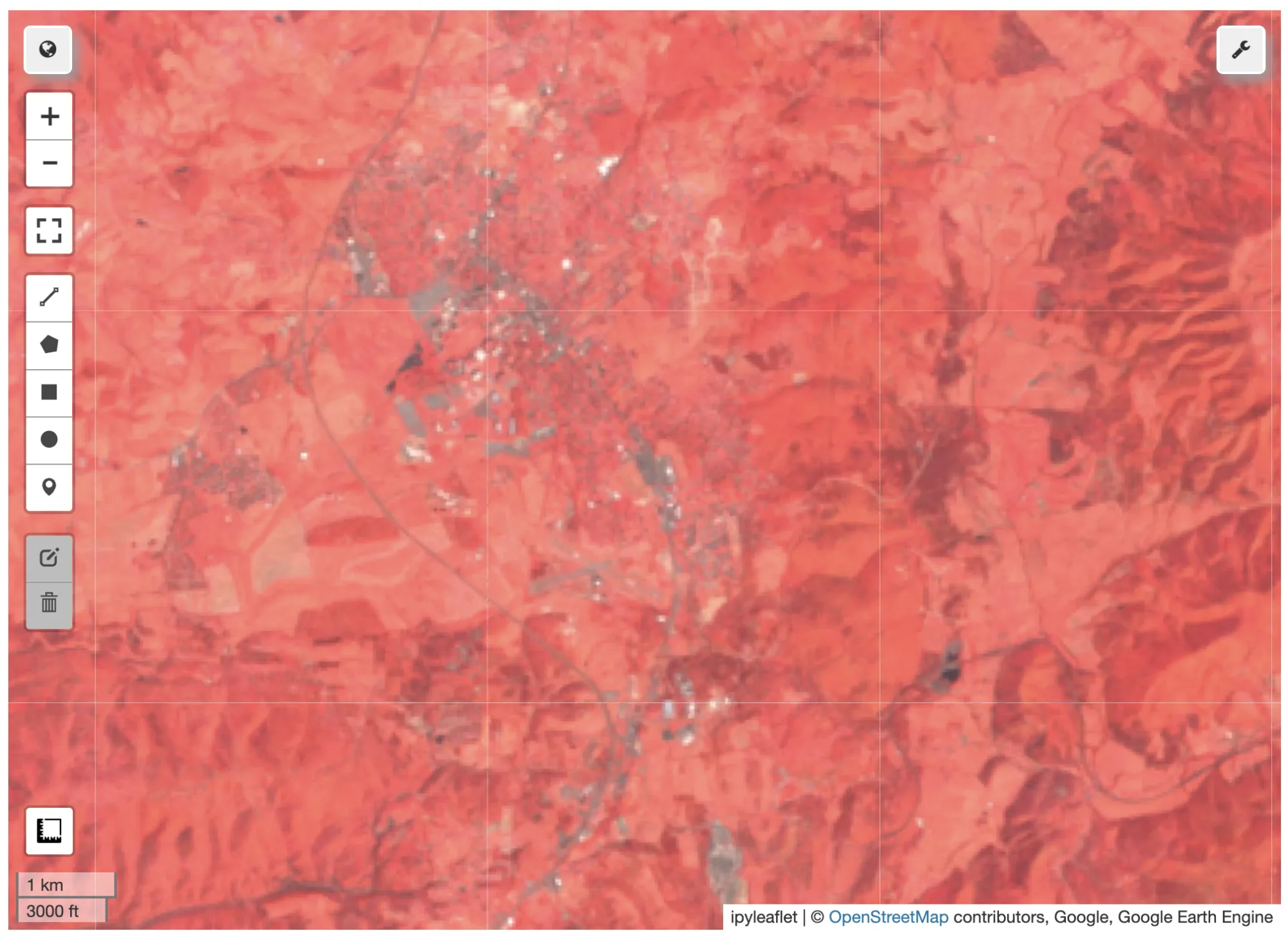
Question 2: By assigning the NIR, red, and green bands to RGB (4-3-2), what features appear bright red in a Landsat 5 image and why? Explore water bodies, urban centers, farms and forests to find relationships between the bands.

Sentinel

The Copernicus Program is a European initiative that is run by the European Space Agency (ESA) in partnership with the European Commission. Its aim is to provide accurate, timely, and easily accessible information to improve the management of the environment, understand and mitigate the effects of climate change, and ensure civil security. A cornerstone of this program is the Sentinel satellite constellation, which collects high-resolution optical and Synthetic Aperture Radar (SAR) imagery globally. The Sentinel satellites are designed to deliver a wealth of data and imagery that can be used for a wide range of applications, including land and water monitoring, emergency response, and climate change research. Sentinel-1 provides all-weather, day-and-night radar images, while Sentinel-2 offers high-resolution optical images with 10m spatial resolution for detailed observation of land cover, agriculture, and forestry. These capabilities make Sentinel a critical tool for environmental monitoring and management, providing vital data for both scientific research and practical applications.

var lat = 37.22; var lon = -80.42; var zoom = 14
var image = (
    ee.ImageCollection('COPERNICUS/S2_SR_HARMONIZED')
         .filterBounds(ee.Geometry.Point(lon, lat))
         .filterDate('2019-01-01', '2019-12-31')
         .sort('CLOUDY_PIXEL_PERCENTAGE')
         .first()
)
var bands = ['B4', 'B3', 'B2']
var vizParams = {
    'bands': bands, 
    'min': 0, 
    'max': 3300
}
Map.setCenter(lon, lat, zoom);
Map.addLayer(image, vizParams, 'Sentinel');

lat = 37.22; lon = -80.42; zoom = 14
image = (
    ee.ImageCollection('COPERNICUS/S2_SR_HARMONIZED')
         .filterBounds(ee.Geometry.Point(lon, lat))
         .filterDate('2019-01-01', '2019-12-31')
         .sort('CLOUDY_PIXEL_PERCENTAGE')
         .first()
)
bands = ['B4', 'B3', 'B2']
vizParams = {
    'bands': bands, 
    'min': 0, 
    'max': 3300
}
map = build_map(lat, lon, zoom, vizParams, image, 'Sentinel')
map

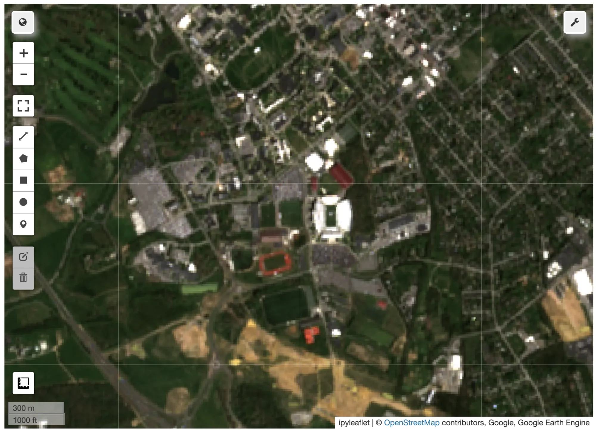
High Resolution Data

Very high resolution data exists, but in many cases, it is not widely available for free. Companies such as Planet Labs and Maxar operate satellites capable of collecting imagery in the sub-meter resolution range. Academics may be able to obtain sample data, but it is not openly available to the public.

The National Agriculture Imagery Program (NAIP) is an effort by the USDA to acquire imagery over the continental US on a multi-year cycle (every three years since 2009, according to the Earth Engine catalog) using airborne sensors (aircraft as opposed to satellites). Because aircraft are much closer to land than satellites (and do not deal with as many atmospheric effects), NAIP imagery is acquired at a ground sample distance of about 1 meter (the catalog notes that some older images are 2 meters). This is considered ‘high resolution data’.

Since NAIP imagery is distributed as ‘quarters’ of Digital Ortho Quads at irregular intervals, load everything from 2012 and mosaic() the images together for display.

var lat = 37.22; var lon = -80.42; var zoom = 14
var image = (
    ee.ImageCollection("USDA/NAIP/DOQQ")
         .filterBounds(ee.Geometry.Point(lon, lat))
         .filterDate('2012-01-01', '2012-12-31')
)
var bands = ['R', 'G', 'B']
var vizParams = {
    'bands': bands, 
    'min': 0, 
    'max': 255
}
Map.setCenter(lon, lat, zoom);
Map.addLayer(image.mosaic(), vizParams, 'NAIP');

lat = 37.22; lon = -80.42; zoom = 14
image = (
    ee.ImageCollection("USDA/NAIP/DOQQ")
         .filterBounds(ee.Geometry.Point(lon, lat))
         .filterDate('2012-01-01', '2012-12-31')
)
bands = ['R', 'G', 'B']
vizParams = {
    'bands': bands, 
    'min': 0, 
    'max': 255
}
map = build_map(lat, lon, zoom, vizParams, image.mosaic(), 'NAIP')
map

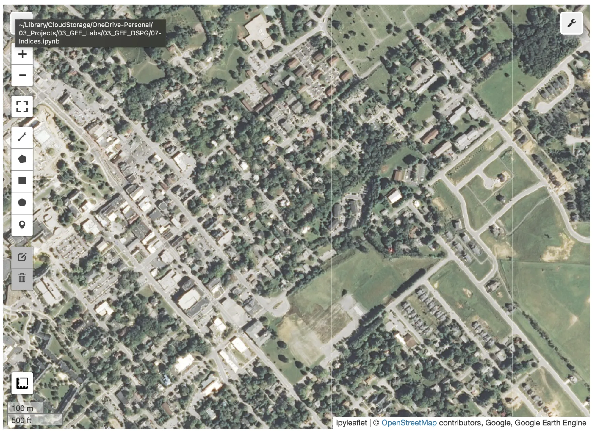
Look at the difference in the resolution - with Landsat and MODIS, each pixel could broadly identify the land type, but NAIP imagery has very high resolution - you can see individual parked cars, the outline of small trees, building envelopes, etc. Start asking yourself how the spatial resolutions of different platforms could help you answer unique questions.

Check the scale of NAIP by getting the first image from the collection (images within a mosaic might have different projections) and getting its scale (meters).

// Get the NAIP resolution from the first image in the collection.
var naipScale = ee.Image(image.first()).
              projection().nominalScale();   
print('NAIP scale:', naipScale);

naipScale = (ee.Image(image.first()).
              projection().nominalScale());   
print('NAIP scale:', naipScale.getInfo());

Question 3: The NAIP imagery above is from 2012. What is the scale of the most recent year of NAIP imagery available in the Earth Engine catalog for the area around Blacksburg, VA? How did you determine the scale?

Temporal Resolution

Temporal resolution refers to the revisit time, or how often the same satellite platform covers the same place on Earth. Historically, satellites have been large, solitary objects that had to make tradeoffs between spatial and temporal resolution. For example, MODIS measures wide swathes of land with each sweep and has relatively high temporal resolution. In contrast, Landsat has improved spatial resolution but a revisit rate of 16 days, and NAIP imagery is acquired on a multi-year cycle.

Over the past decade, satellite technology has improved, and there is more diversity in mission sets. Cube satellites are small, shoe-box-sized satellites that can provide both high-resolution imagery and, when mosaiced together, provide high temporal resolution as well. The tradeoff is that these satellites do not have the same array of sophisticated sensors that larger satellites are equipped with. Other satellites, such as those run by the intelligence community and private satellite companies, are designed for rapid revisit times of certain cities or political areas while not scanning the rest of the world.

Understanding and considering temporal resolution for your use case is crucial, as there are tradeoffs to be made either way.

Resolution of a few popular platforms:

1. Landsat: 16 days
2. MODIS: Several satellites, temporal resolution varies by product (4 days to annual products)
3. Sentinel: 5 days at the equator
4. NAIP: 3-year cycle (since 2009)
5. Planet: Daily

Landsat (5 and later) produces imagery at a 16-day cadence. TM and MSS are on the same satellite (Landsat 5), so you can print the TM series to see the temporal resolution. Unlike MODIS, data from these sensors is produced on a scene basis, so to see a time series, it’s necessary to filter by location in addition to time. If the list skips expected 16-day dates, some scenes may be missing from the collection, for example because of quality control.

While you can look at the date ranges in the filename or expand each image in the list to look at the DATE_ACQUIRED property, there is a better way to extract this information programmatically. In this case, we are building a function within JavaScript to extract the date and time from each image.

var lat = 37.22; var lon = -80.42; var zoom = 14
// Filter to get a year's worth of TM scenes.
var tmSeries = ee.ImageCollection("LANDSAT/LT05/C02/T1_TOA")
  .filterBounds(ee.Geometry.Point(lon, lat))
  .filterDate('2011-01-01', '2011-12-31');

// Build a function called getDate
var getDate = function(image) {
// Note that you need to cast the argument
  var time = ee.Image(image).get('system:time_start');
// Return the time (in milliseconds since Jan 1, 1970) as a Date
  return ee.Date(time);
};
var dates = tmSeries.toList(100).map(getDate);
print(dates)

lat = 37.22; lon = -80.42; zoom = 14
# Filter to get a year's worth of TM scenes.
tmSeries = (ee.ImageCollection("LANDSAT/LT05/C02/T1_TOA")
  .filterBounds(ee.Geometry.Point(lon, lat))
  .filterDate('2011-01-01', '2011-12-31'));

# Build a function called getDate
def getDate(image):
    # Note that you need to cast the argument
    time = ee.Image(image).get('system:time_start')
    # Return the time (in milliseconds since Jan 1, 1970) as a Date
    return ee.Date(time)
dates = tmSeries.toList(100).map(getDate);
print(dates.getInfo())

Question 4: What is the temporal resolution of the Sentinel-2 satellites? How can you determine this?

Spectral Resolution

Spectral resolution refers to the number and width of spectral bands in which the sensor takes measurements. You can think of the width of spectral bands as the wavelength interval on the electromagnetic spectrum for each band. A sensor that measures radiance in multiple bands (e.g., collects a value for red, green, blue, and near-infrared) is called a multispectral sensor (generally 3-10 bands), while a sensor with many bands (possibly hundreds) is called a hyperspectral sensor (these are not hard and fast definitions). For example, compare the multispectral OLI aboard Landsat 8 to Hyperion, a hyperspectral sensor that collects 220 unique spectral channels aboard the EO-1 satellite.

You will have to read through the documentation for each image collection to understand the spectral response of the bands.

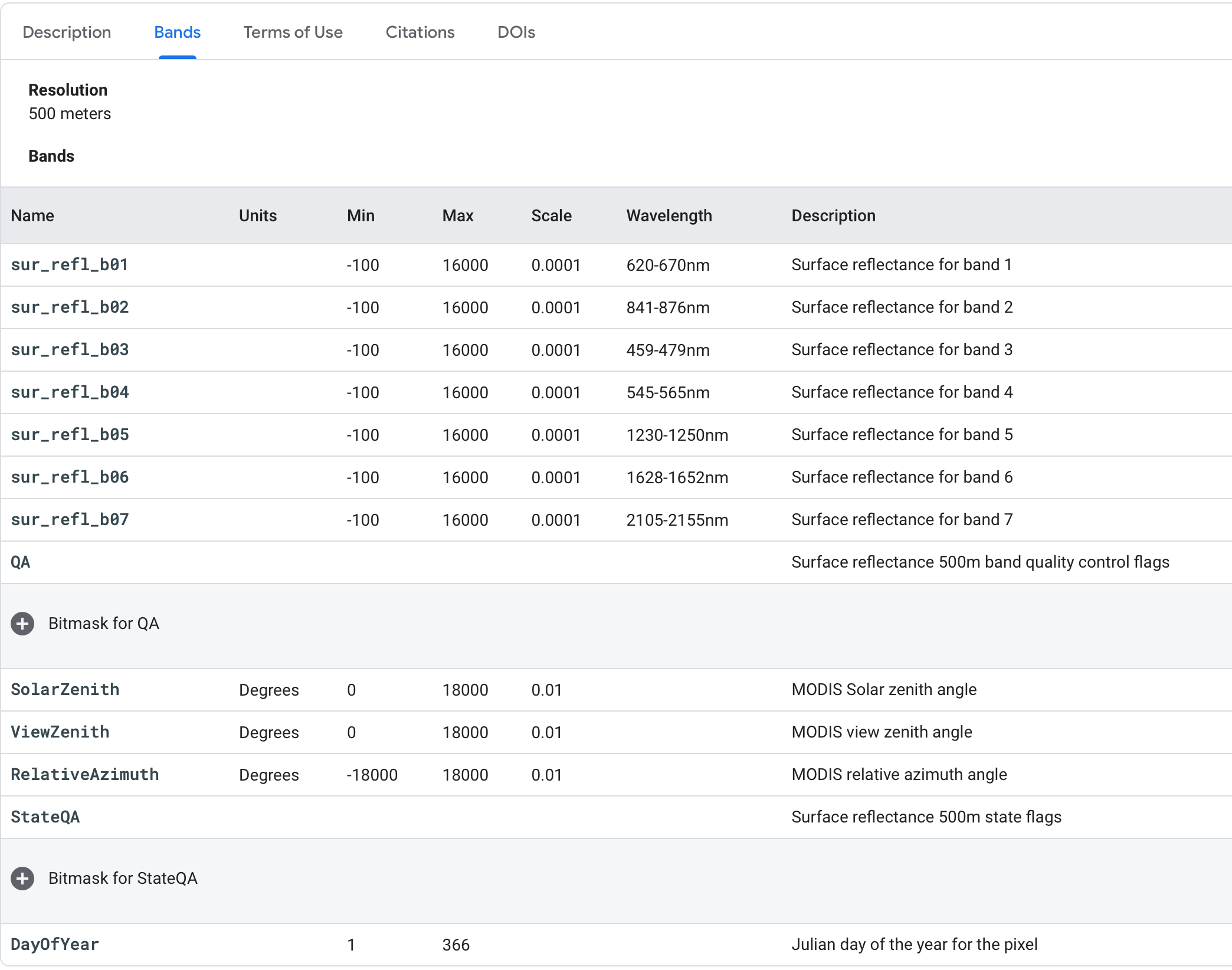
Note: Not all bands contain radiometric data. Some are quality control data, while others include information about the zenith or cloud coverage. You can use these other bands to either mask out low-quality pixels or conduct additional calculations. It is a good idea to read through the documentation of each dataset you will be working with to get a good understanding of the band structure.

You can use the code below to check the number of bands in Earth Engine, but you will have to read through the documentation for each image collection to understand the spectral response of the bands.

To see the number of bands in an image, use:

var dataset = ee.ImageCollection('MODIS/061/MOD09A1')
                  .filter(ee.Filter.date('2018-01-01', '2018-05-01'))
                  .first();
// Get the MODIS band names as a List
var modisBands = dataset.bandNames();
// Print the list.
print('MODIS bands:', modisBands);
// Print the length of the list.
print('Length of the bands list:', modisBands.length());

dataset = (ee.ImageCollection('MODIS/061/MOD09A1')
                  .filter(ee.Filter.date('2018-01-01', '2018-05-01'))
                  .first())
# Get the MODIS band names as a List
modisBands = dataset.bandNames();
# Print the list.
print('MODIS bands:', modisBands.getInfo());
#  Print the length of the list.
print('Length of the bands list:', modisBands.length().getInfo());

Question 5: What is the spectral resolution of the MODIS instrument? How did you determine it?

Question 6: Investigate the bands available for the USDA NASS Cropland Data Layers (CDL). What do the individual bands within the CDL represent? Which band(s) would you select if you were interested in evaluating the extent of pasture areas in the US?

Radiometric Resolution

Radiometric resolution refers to the value, or ‘digital number’ that the sensor records: coarse radiometric resolution would record a scene with only a narrow range of values, whereas fine radiometric resolution would record the same scene using a wide range of values. The precision of the sensing, or the level of quantization, is another way to refer to radiometric resolution. 8-bit values (0-255) are standard in many image processing tools.

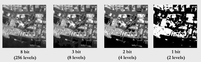
Radiometric resolution is determined from the minimum radiance to which the detector is sensitive (L_min), the maximum radiance at which the sensor saturates (L_max), and the number of bits used to store the DNs (Q):

Radiometric resolution = (L_max - L_min) / 2^Q

It might be possible to dig around in the metadata to find values for L_min and L_max, but computing radiometric resolution is generally not necessary unless you’re studying phenomena that are distinguished by very subtle changes in radiance. One thing to keep in mind is that while sensors have developed and become more sensitive/accurate, capable of recording data in upwards of 16 bits, that may not necessarily be beneficial for your work. Computation and storage costs grow, and normalizing the data to 8-bit values to work with tools such as OpenCV defeats the purpose of this sensitive collection rate. There are use cases where high bit rate collection makes sense (e.g., looking for a very narrow range in a custom spectral range to identify mineral deposits), but ensure that you understand where and why higher radiometric resolution is necessary.

Digital Image Visualization and Stretching

You’ve learned about how an image stores pixel data in each band as digital numbers (DNs) and how the pixels are organized spatially. When you add an image to the map, Earth Engine handles the spatial display for you by recognizing the projection and putting all the pixels in the right place. However, you must specify how to stretch the DNs to fit the standard 8-bit display image that GEE uses (min and max parameters). Specifying min and max applies (where DN’ is the displayed value):

DN’ = 255 * (DN - min) / (max - min)

For instance, if you are working with NAIP imagery, you can set the display min to 0 and max to 255 to model 8-bit radiometric resolution.

var lat = 37.22; var lon = -80.42; var zoom = 14
var image = (
    ee.ImageCollection("USDA/NAIP/DOQQ")
         .filterBounds(ee.Geometry.Point(lon, lat))
         .filterDate('2012-01-01', '2012-12-31')
)
var bands = ['R', 'G', 'B']
var vizParams = {
    'bands': bands, 
    'min': 0, 
    'max': 255
}
Map.setCenter(lon, lat, zoom);
Map.addLayer(image, vizParams, 'NAIP');

lat = 37.22; lon = -80.42; zoom = 14
image = (
    ee.ImageCollection("USDA/NAIP/DOQQ")
         .filterBounds(ee.Geometry.Point(lon, lat))
         .filterDate('2012-01-01', '2012-12-31')
)
bands = ['R', 'G', 'B']
vizParams = {
    'bands': bands, 
    'min': 0, 
    'max': 255
}
map = build_map(lat, lon, zoom, vizParams, image, 'NAIP')
map

By contrast, the Planet MultiSpectral SkySat imagery uses 16 bit collection, so you have to adjust the min and max values. If your image is not displaying correctly (such as a black screen) check the documentation for your data and adjust your min and max values.

var dataset = ee.ImageCollection('SKYSAT/GEN-A/PUBLIC/ORTHO/MULTISPECTRAL');
var bands = ['N', 'G', 'B'];
var vizParams = {
  bands: bands,
  min: 200.0,
  max: 6000.0,
};
Map.setCenter(-70.892, 41.6555, 15);
Map.addLayer(dataset, vizParams, 'Planet Labs');

image = ee.ImageCollection('SKYSAT/GEN-A/PUBLIC/ORTHO/MULTISPECTRAL');
bands = ['N', 'G', 'B']
vizParams = {
    'bands': bands, 
    'min': 200, 
    'max': 6000 
}
lat = 41.6555; lon = -70.892; zoom = 15
map = build_map(lat, lon, zoom, vizParams, image, 'Planet Labs')
map

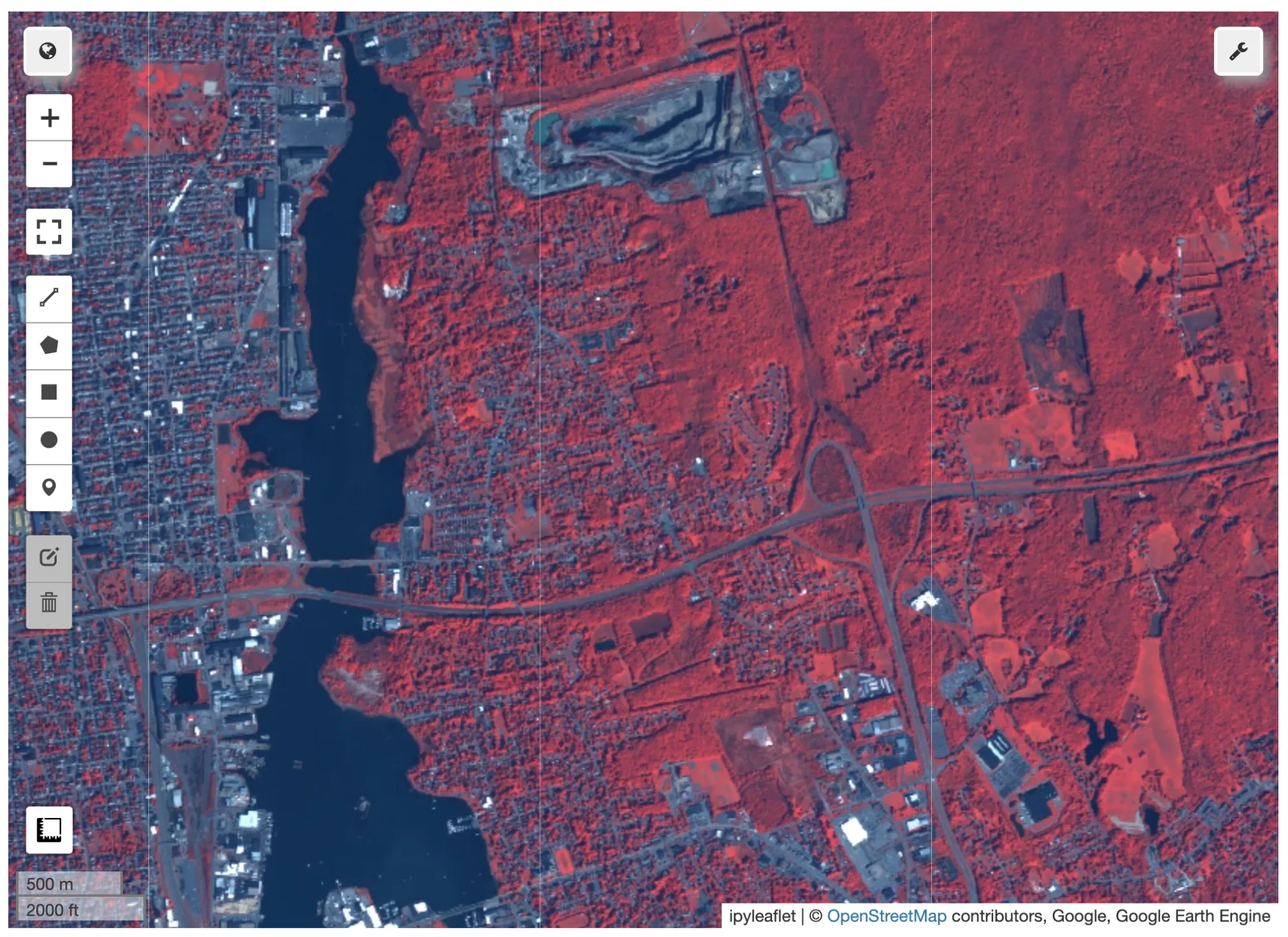
Resampling and ReProjection

Earth Engine makes every effort to handle projection and scale so that you don’t have to. However, there are occasions where an understanding of projections is important to get the output you need. Earth Engine requests inputs to your computations in the projection and scale of the output. The map panel in the Code Editor uses a Mercator projection.

The scale is determined from the map’s zoom level. When you add something to this map, Earth Engine secretly reprojects the input data to Mercator, resampling (with nearest neighbor) to the screen resolution pixels based on the map’s zoom level, then does all the computations with the reprojected, resampled imagery. None of the examples on this page call reproject(); a reproject() call forces the computation to be done in the projection and scale you pass to it instead of the map’s.

If you are familiar working with remote sensing data in another programming language, such as R or Python, you have to deal with projections and resampling on your own. Google Earth Engine takes care of this behind the scenes, which simplifies your work. We mention it here because this is a change when starting to use GEE. A more thorough discussion about projections is in the documentation.