Transformations
Code status: The code on this page was corrected on 17 September 2026 against the current Earth Engine Data Catalog and API documentation. It has not been executed against Earth Engine. Screenshots, printed values and described outputs come from earlier versions of this lesson and may differ from what the corrected code produces.
We’ve gone over indices to highlight unique characteristics in our imagery by utilizing the bands outside of the visible spectrum.
3B.1 - Band Transforms
Linear transforms are linear combinations of input pixel values. These can result from a variety of different strategies, but a common theme is that pixels are treated as arrays of band values, and we can use these arrays to create weighted values for specific purposes. The last transform in this section, HSV, is a non-linear change of color space.
3B.1.1 - Tasseled cap (TC)
Based on observations of agricultural land covers in the NIR-red spectral space, Kauth and Thomas (1976) devised a rotational transform of the form
$$p_1 = R^T p_0$$
where:
$p_0$ is the original pixel vector (a stack of the p band values as an Array)
$p_1$ is the rotated pixel
R is an orthonormal basis of the new space (inverse of $R^T$). Kauth and Thomas found R by defining the first axis of their transformed space to be parallel to the soil line in the following chart, then used the Gram-Schmidt process to find the other basis vectors.
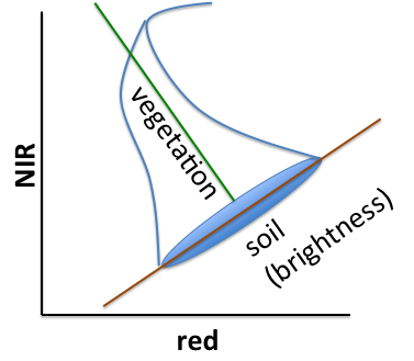
Assuming that R is available, one way to implement this rotation in Earth Engine is with arrays. Specifically, make an array of TC coefficients. Since these coefficients are for the TM sensor, get a less cloudy Landsat 5 scene. To do the matrix multiplication, first convert the input image from a multi-band image to an array image in which each pixel position stores an array. Do the matrix multiplication, then convert back to a multi-band image.
Python setup: every Python cell on this page assumes this block has already run in the same session. Registering a Cloud project and authenticating are covered in Getting Started with Earth Engine.
# opens the sign-in flow when no stored credentials exist
# use your registered Cloud project ID
=
return
;
;
;
;
// Make an Array Image, with a 1-D Array per pixel.
;
// Make an Array Image with a 2-D Array per pixel, 6x1.
;
arrayImage2D
// Get rid of the extra dimensions.
// Get a multi-band image with TC-named bands.
;
;
point, 9
componentsImage, vizParams, 'TC components';
= 39.19; = -106.81;
= 9
=
=
=
=
=
=
= ;
=
# Make an Array Image, with a 1-D Array per pixel.
= ;
# Make an Array Image with a 2-D Array per pixel, 6x1.
= ;
=
=
=
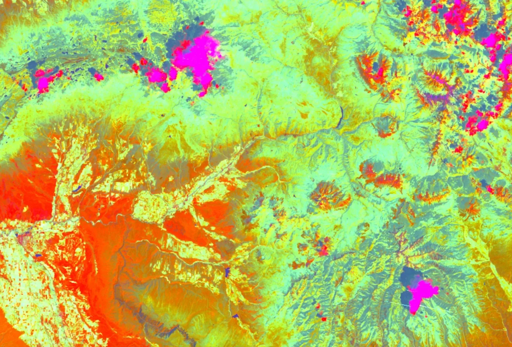
Question 3: Change the point in the code to a location near Blacksburg, VA, produce a tasseled cap image there and interpret the output. What are some of the values that you can extract when using Inspector? Are the results meaningful?
3B.1.2 - Principal Component Analysis (PCA)
Like the Tasseled Cap transform, the PCA transform is a rotational transform in which the new basis is orthonormal, but the axes are determined from statistics of the input image, rather than fixed, sensor-specific coefficients. Specifically, the new basis is the eigenvector of the image’s variance-covariance matrix. As a result, the principal components are uncorrelated. To demonstrate, use the reflective bands of a Landsat 8 image (B2 to B7). The thermal bands are left out because they are in kelvin rather than reflectance, and in an unstandardised covariance their much larger values would dominate the first component. Following the Earth Engine Eigen analysis guide, first mean-centre each band by subtracting its mean over the scene, then convert the centred image to an array image. Use the reduceRegion() method to compute statistics (band covariances) for the image.
A reducer is an object that tells Earth Engine what statistic to compute. Note that the result of the reduction is an object with one property, an array, that stores the covariance matrix. The next step is to compute the eigenvectors and eigenvalues of that covariance matrix. Since the eigenvalues are prepended to the eigenvectors, slice the two apart and keep the eigenvectors, discarding the eigenvalues (column 0). Perform the matrix multiplication, as with the TC components. Finally, convert back to a multi-band image and display the first PC.
Use the layer manager described in the Earth Engine Code Editor guide to stretch the result appropriately. What do you observe? Try displaying some of the other principal components. The code chunk below displays only Principal Component 1, with no stretch set, so choose the minimum and maximum in the layer manager.
;
;
// Reflective bands only: the thermal bands are in kelvin, not reflectance.
;
;
// Mean-centre each band by subtracting its mean over the scene.
;
;
;
;
;
;
;
;
;
// Make the one band array image a multi-band image, [] -> image.
;
// Display PC1; set the stretch in the layer manager.
point, 10;
'pc1', , 'PC1';
= 37.22; = -80.42;
= 10
=
=
=
=
=
=
# Reflective bands only: the thermal bands are in kelvin, not reflectance.
=
=
# Mean-centre each band by subtracting its mean over the scene.
=
=
=
=
=
= ;
= ;
= ;
= ;
= ;
# Display PC1; set the stretch in the layer control.
=
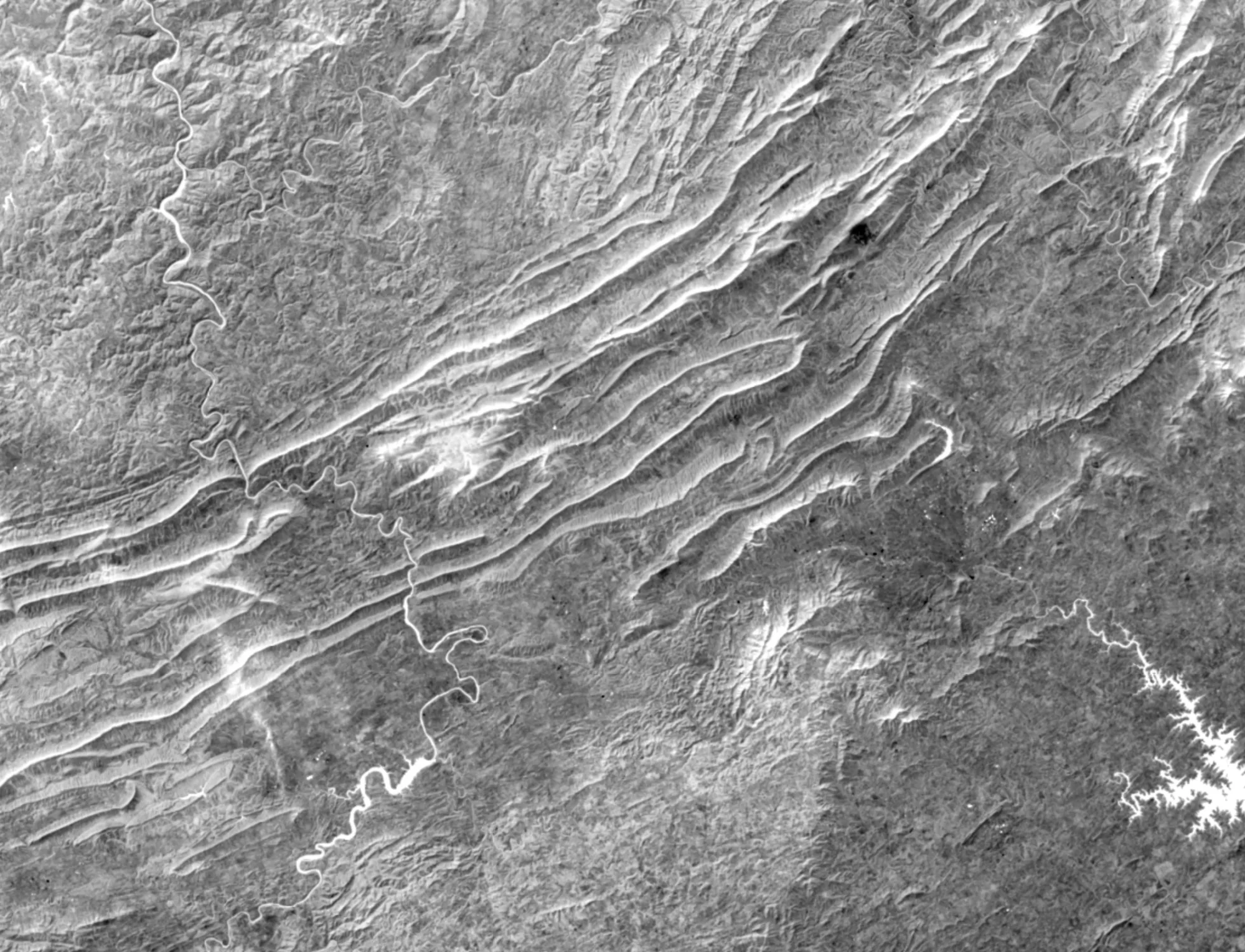
Question 4: How much did you need to stretch the results to display outputs for principal component 2?
Display and describe images of each of the other principal components, stretching each band as needed for visual interpretation and indicating how you selected the min and max values.
How do you interpret each PC band? On what basis do you make that interpretation?
3B.1.3 - Spectral Unmixing
The linear spectral mixing model is based on the assumption that each pixel is a mixture of “pure” spectra. The pure spectra, called endmembers, are from land cover classes such as water, bare land, vegetation. The goal is to solve the following equation for f, the Px1 vector of endmember fractions in the pixel:
$$Sf = p$$
where S is a BxP matrix in which the columns are P pure endmember spectra (known) and p is the Bx1 pixel vector when there are B bands (known). In this example, $B= 6$:
The first step is to get the endmember spectra, which we can do by computing the mean spectra in polygons around regions of pure land cover. In this example, we will use a location in northern Washington State and use the geometry tools to select homogeneous areas of bare land, vegetation and water.
Using the geometry drawing tools described in the Earth Engine Code Editor guide, make three layers clicking + new layer. In the first layer, digitize a polygon around pure bare land, in the second layer make a polygon of pure vegetation, and in the third layer, make a water polygon. Name the imports bare, vegetation and water, respectively.
Note: For a starting point, we included some basic polygons but feel free to replace in a region of your choice.
;
;
// Polygons of bare earth, water and vegetation
;
;
;
;
= 48.11; = -123.25;
= 11
=
=
=
=
=
=
# Polygons of bare earth, water and vegetation
=
=
=
=
Check the polygons you made by charting mean spectra in them using ui.Chart.image.regions(). The Python tab computes the same means with reduceRegions() and plots them with matplotlib.
;
unmixImage, ,
, 30, 'label',;
=
=
=
=
Use the reduceRegion() method to compute mean spectra in the polygons you made. Note that the return value of reduceRegion() is a Dictionary, with reducer output keyed by band name. Get the means as a list by calling values(). Each of these three lists represents a mean spectrum vector. Stack the vectors into a 6x3 Array of endmembers by concatenating them along the 1-axis (or columns direction).
Turn the 6-band input image into an image in which each pixel is a 1D vector (toArray()), then into an image in which each pixel is a 6x1 matrix (toArray(1)). Now that the dimensions match, in each pixel, solve the equation for f. Finally, convert the result from a 2D array image into a 1D array image (arrayProject()), then to a multi-band image (arrayFlatten()). The three bands correspond to the estimates of bare, vegetation and water fractions in f. Display the result where bare is red, vegetation is green, and water is blue (the addLayer() call expects bands in order, RGB)
;
;
;
;
;
;
;
;
point, 11
unmixedImage, , 'Unmixed';
= ;
= ;
= ;
= ;
= ;
= ;
= ;
=
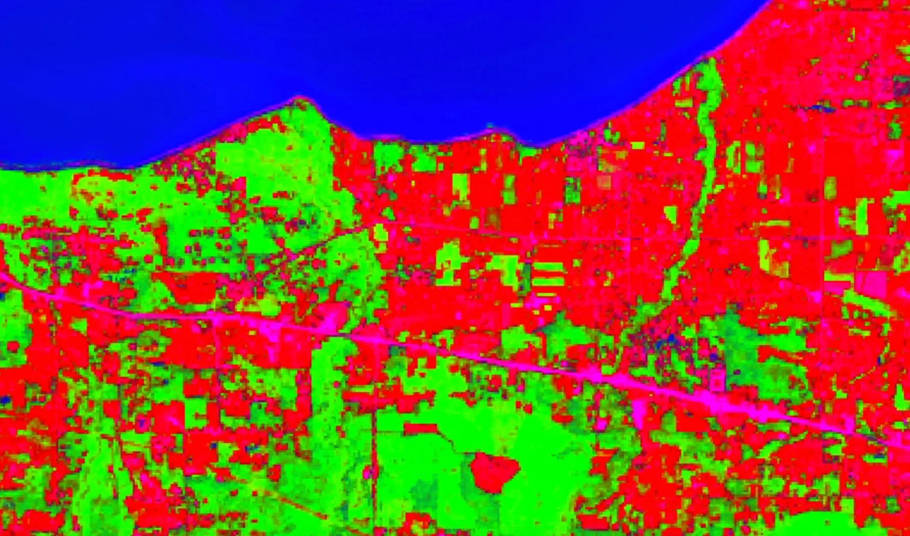
Question 5: Repeat this process for Blacksburg, VA. Produce the mean spectra chart for bare, water, and land and the unmixed map, and describe them. Interpret the output of the image by selecting different pixels with Inspector.
3B.1.4 - Hue-Saturation-Value Transform
The Hue-Saturation-Value (HSV) model is a color transform of the RGB color space. Among many other things, it is useful for pan-sharpening. This involves converting an RGB to HSV, swapping the panchromatic band for the value (V), then converting back to RGB. For example, using the Landsat 8 scene:
;
;
// Convert Landsat RGB bands to HSV
;
// Convert back to RGB, swapping the image panchromatic band for the value.
;
point, 12;
rgb, , 'Pan-sharpened';
= 37.22; = -80.42;
= 12
=
=
=
=
=
=
# Convert Landsat RGB bands to HSV
= ;
# Convert back to RGB, swapping the image panchromatic band for the value.
= ;
=
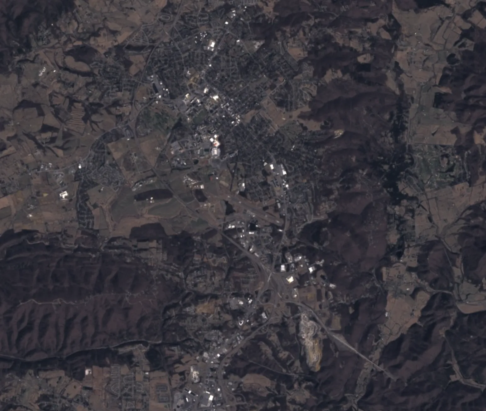
Question 6: Compare the pan-sharpened image with the original image. What do you notice that’s different? The same?
3B.2 - Spectral Transformation
3B.2.1 - Linear Filtering
In the present context, linear filtering (or convolution) refers to a linear combination of pixel values in a ‘neighborhood’, or kernel, where the weights of the kernel determine the coefficients in the linear combination (on this page, the terms kernel and filter are interchangeable.) Filtering an image can be useful for extracting image information at different spatial frequencies: suppressing high frequencies reduces noise, while emphasising them highlights edges. For this reason, smoothing filters are called low-pass filters (they let low-frequency data pass through) and edge detection filters are called high-pass filters. To implement filtering in Earth Engine use image.convolve() with an ee.Kernel for the argument.
3B.2.2 - Smoothing
Smoothing means to convolve an image with a smoothing kernel.
A simple smoothing filter is a square kernel with uniform weights that sum to one. Convolving with this kernel sets each pixel to the mean of its neighborhood. Print a square kernel with uniform weights (this is sometimes called a “pillbox” or “boxcar” filter):
Expand the kernel object in the console to see the weights. This kernel is defined by how many pixels it covers (i.e. radius is in units of ‘pixels’). A kernel with radius defined in ‘meters’ adjusts its size in pixels, so you can’t visualize its weights, but it’s more flexible in terms of adapting to inputs of different scale. In the following, use kernels with radius defined in meters except to visualize the weights.
;
;
// Print a uniform kernel to see its weights.
'A uniform kernel:', 2;
= 37.22; = -80.42;
= 12
=
=
=
=
=
=
# Print a uniform kernel to see its weights.
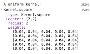
Define a kernel with 2-meter radius (which corresponds to how many pixels in the NAIP image? Hint: try projection.nominalScale()), convolve the image with the kernel and compare the input image with the smoothed image:
// Define a square, uniform kernel.
;
// Filter the image by convolving with the smoothing filter.
;
;
point, 12;
smoothed, trueColorVis, 'smoothed image';
# Define a square, uniform kernel.
=
# Filter the image by convolving with the smoothing filter.
=
=
=
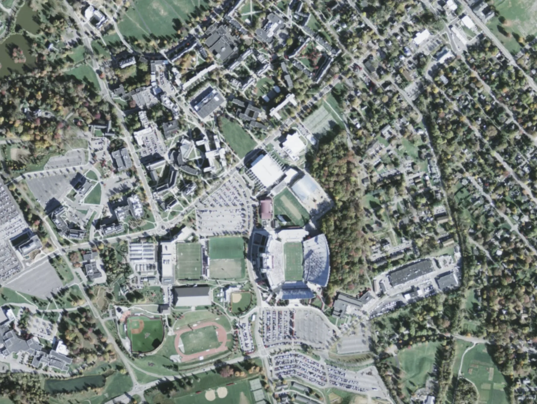
To make the image even smoother, try increasing the size of the neighborhood by increasing the pixel radius. To the human eye, the image is blurrier, but in many Machine Learning and Computer Vision algorithms, this process improves our output by reducing noise.
A Gaussian kernel can also be used for smoothing. Think of filtering with a Gaussian kernel as computing the weighted average in each pixel’s neighborhood.
// Print a Gaussian kernel to see its weights.
'A Gaussian kernel:', 2;
// Define a square Gaussian kernel:
;
// Filter the image by convolving with the Gaussian filter.
;
;
point, 12;
gaussian, trueColorVis, 'smoothed image';
# Print a Gaussian kernel to see its weights.
# Define a square Gaussian kernel:
=
# Filter the image by convolving with the Gaussian filter.
=
=
Question 7: What happens as you increase the pixel radius for each smoothing? What differences can you discern between the weights and the visualizations of the two smoothing kernels?
3B.2.3 - Edge Detection
Convolving with an edge-detection kernel is used to find rapid changes in values that usually signify the edges of objects in the image data.
A classic edge detection kernel is the Laplacian kernel. Investigate the kernel weights and the image that results from convolving with the Laplacian. Other edge detection kernels include the Sobel, Prewitt and Roberts kernels. Learn more about additional edge detection methods in Earth Engine.
;
;
// Define a Laplacian, or edge-detection kernel.
;
// Apply the edge-detection kernel.
;
;
point, 12;
edges, trueColorVis,'edges';
# Define a Laplacian, or edge-detection kernel.
=
# Apply the edge-detection kernel.
=
=
=
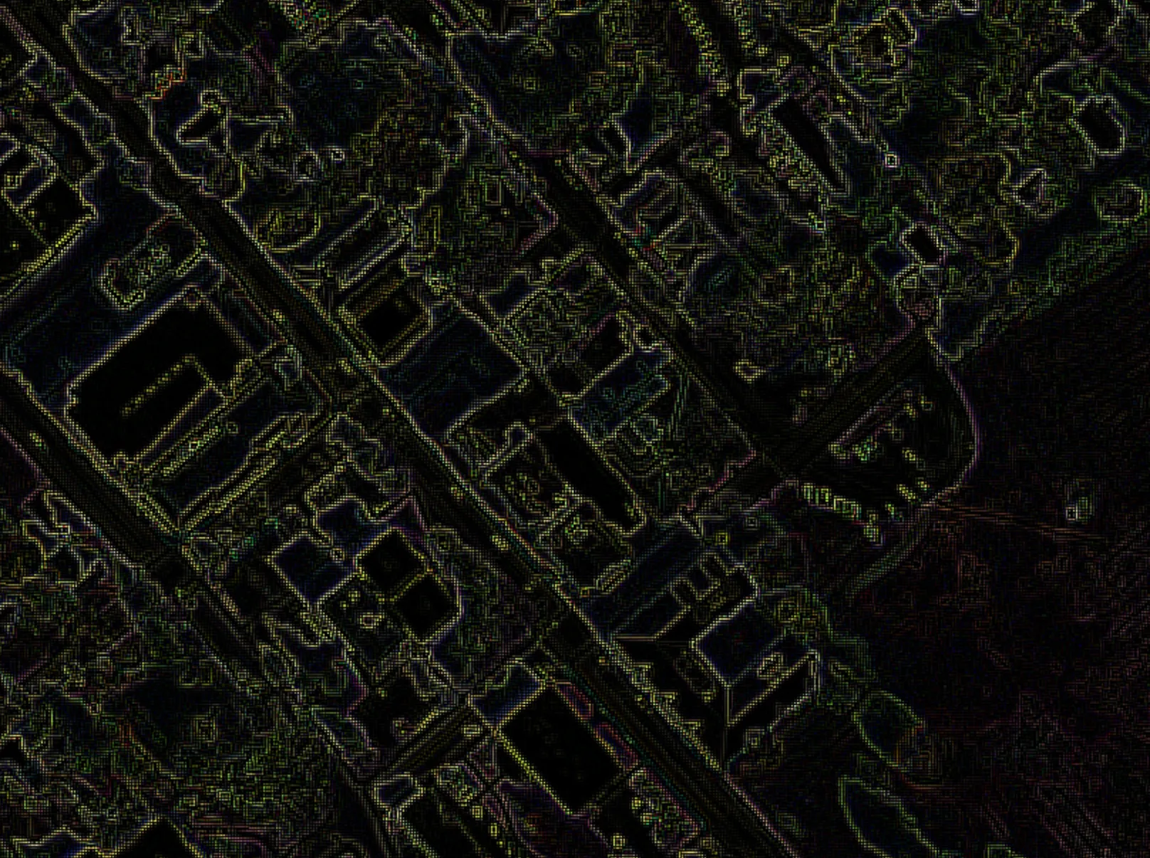
Question 8: Choose another edge detection method, produce the image and describe it: what characteristics do you see, and how does it compare to Laplacian edge detection?
Additional Exercises
Question 9: Look in google scholar to identify 2-3 publications that have used NDVI and two-three that used EVI. For what purposes were these indices used and what was the justification provided for that index?
Question 10: Discuss a spectral index that is not covered on the Indices page and relates to your area of research/interest. What is the name of the spectral index, the formula used to calculate it, and what is it used to detect? Provide a citation of an academic article that has fruitfully used that index.
Question 11: Find 1-2 articles that use any of the linear transformation methods practised on this page in the service of addressing an important social issue (e.g., one related to agriculture, environment, or development). Provide the citations and discuss how the transformation is used and how it’s justified in the article.