Visualizing Images

Code status: The code on this page was corrected on 17 September 2026 against the current Earth Engine Data Catalog and API documentation. It has not been executed against Earth Engine. Screenshots, printed values and described outputs come from earlier versions of this lesson and may differ from what the corrected code produces.

In this lab, we will search for and visualize imagery in Google Earth Engine. We will discuss the difference between radiance and reflectance, make true color and false color composites from different bands and visually identify land cover types based on characteristics from the imagery. We will also discuss atmospheric effect on data collection by looking at the different data products available.

Learning Outcomes

• Extract single scenes from collections of images
• Create and visualize true color and false color composites
• Use the Inspector tab to assess pixel values
• Understand the difference between radiance and reflectance through visualization

2.2 - Searching for Imagery

The Landsat program is a joint program between NASA and the United States Geological Survey (USGS) that has launched a sequence of Earth observation satellites (Landsat 1-9). Originating in 1972, the Landsat program provides the longest continuous observation of the Earth’s surface. Take the time to monitor some of the fascinating timelapses using Landsat to showcase things like urban development, glacial retreat and deforestation.

Let’s load a Landsat scene over our region of interest, inspect the units and plot the radiance. Specifically, use imagery from Landsat 8. Landsat 9 Collection 2 data are also in the Earth Engine catalog (for example LANDSAT/LC09/C02/T1_TOA), but this lab uses Landsat 8 throughout.

To inspect a Landsat 8 image (also called a scene) in our region of interest (ROI), we can choose a point to center our map, filter the image collection to get a scene with few clouds, and display information about the image in the console.

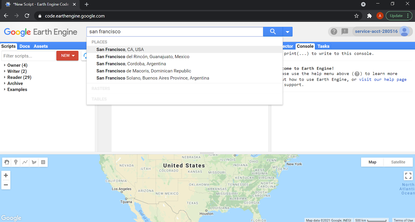
You can either scroll to the area on the map you’re interested in and choose a point or use the search bar to find your location. Use the geometry tool to make a point near Blacksburg, VA (for these exercises we will include the point location in the script).

We will be using two USGS Landsat 8 Collection 2 Tier 1 collections: TOA Reflectance in the first code chunk, and Raw Scenes in the chunks that follow. If you read the documentation for the Raw Scenes, the values refer to scaled, calibrated at-sensor radiance. Tier 1 means it is ready for analysis and is the highest quality imagery. There’s quite a bit to learn about how the Landsat data is processed - if you will be working with Landsat extensively, take the time to read the Landsat 8 Data Users Handbook for more information.

We will filter the ImageCollection by date (year 2014) and location (to the ROI, which for this exercise is Blacksburg, VA), sort by a metadata property included in the imagery called CLOUD_COVER and get the first image out of this sorted collection.

Python setup: every Python cell on this page assumes this block has already run in the same session. Registering a Cloud project and authenticating are covered in Getting Started with Earth Engine.

import ee
import geemap

ee.Authenticate()  # opens the sign-in flow when no stored credentials exist
ee.Initialize(project='your-cloud-project-id')  # use your registered Cloud project ID

def build_map(lat, lon, zoom, vis_params, image, name):
    m = geemap.Map(center=[lat, lon], zoom=zoom)
    m.addLayer(image, vis_params, name)
    return m

// Code Chunk 01
var lat = 37.22; var lon = -80.42;
var zoom = 11;
var image_collection_name = "LANDSAT/LC08/C02/T1_TOA";
var date_start = '2014-01-01';
var date_end = '2014-12-31';
var point = ee.Geometry.Point([lon, lat]);

var landsat = ee.ImageCollection(image_collection_name);
//  Note that we need to cast the result of first() to Image.
var image = ee.Image(landsat
                     //  Filter to get only images in the specified range.
                     .filterDate(date_start, date_end)
                     //  Filter to get only images at the location of the point.
                     .filterBounds(point)
                     //  Sort the collection by a metadata property.
                     .sort('CLOUD_COVER')
                     //  Get the first image out of this collection.
                     .first());
//  Print the information to the console
print('A Landsat scene:', image);
var vizParams = {
  bands: ['B4', 'B3', 'B2'],
  min: 0,
  max: 0.4
};
// Add the image to the  map, using the visualization parameters.
Map.setCenter(lon, lat, zoom);
Map.addLayer(image, vizParams, 'true-color image');

# Code Chunk 01
lat = 37.22; lon = -80.42
zoom = 11
image_collection_name = "LANDSAT/LC08/C02/T1_TOA"
date_start = '2014-01-01'
date_end = '2014-12-31'
name = 'true-color image'
point = ee.Geometry.Point([lon, lat])

image = (
    ee.ImageCollection(image_collection_name)
         .filterBounds(point)
         .filterDate(date_start, date_end)
         .sort('CLOUD_COVER')
         .first()
)
print('A Landsat scene:', image.getInfo())

bands = ['B4', 'B3', 'B2']

vizParams = {
    'bands': bands,
    'min': 0,
    'max': 0.4
}

map = build_map(lat, lon, zoom, vizParams, image, name)
map

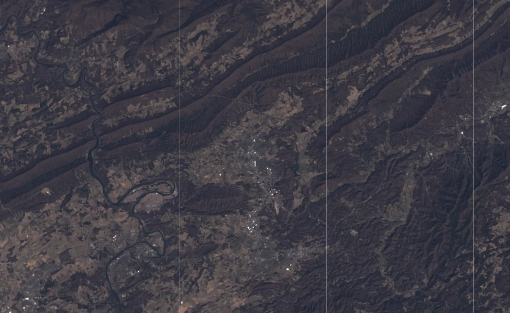
The variable image now stores a reference to an object of type ee.Image. In other words, we have taken the image collection and reduced it down to a single image, which is now ready for visualization.

Before we visualize the data, go to the console and click on the dropdown.

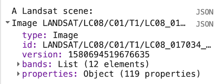
Expand and explore the image by clicking the triangle next to the image name to see more information stored in that object. Specifically, expand properties and inspect the long list of metadata items stored as properties of the image. This is where the CLOUD_COVER property you just used is stored.

There are band specific coefficients (RADIANCE_ADD_BAND_*, RADIANCE_MULT_BAND_* where * is a band number) in the metadata for converting from the digital number (DN) stored by the image into physical units of radiance. These coefficients will be useful in later exercises.

2.3 - Visualizing Landsat Imagery

Recall from Digital Images that Landsat 8 measures radiance in multiple spectral bands. A common way to visualize images is to set the red band to display in red, the green band to display in green and the blue band to display in blue - just as you would create a normal photograph. This means trying to match the spectral response of the instrument to the spectral response of the photoreceptors in the human eye. It’s not a perfect match but this is called a true-color image. When the display bands don’t match human visual perception (as we will see later), the visualization is called a false-color composite.

2.3.1 - True Color Composite

To build a true color image we are building a variable called trueColor that selects the red / green / blue bands in order and includes the min and max value to account for the appropriate radiometric resolution - this piece can be tricky, as it is unique for each dataset you work with. You can find the band names and min-max values to use from the dataset documentation page, but a great starting point is to use the ‘code example’ snippet for each dataset, which will set up the visualization parameters for you.

// Code Chunk 02
var lat = 37.22; var lon = -80.42;
var zoom = 11;
var image_collection_name = "LANDSAT/LC08/C02/T1";
var date_start = '2014-01-01';
var date_end = '2014-12-31';

var point = ee.Geometry.Point([lon, lat]);
var landsat = ee.ImageCollection(image_collection_name);
//  Note that we need to cast the result of first() to Image.
var image = ee.Image(landsat
                     //  Filter to get only images in the specified range.
                     .filterDate(date_start, date_end)
                     //  Filter to get only images at the location of the point.
                     .filterBounds(point)
                     //  Sort the collection by a metadata property.
                     .sort('CLOUD_COVER')
                     //  Get the first image out of this collection.
                     .first());
//  Define visualization parameters in a JavaScript dictionary.
var trueColor = {
  bands: ['B4', 'B3', 'B2'],
  min: 4000,
  max: 18000
};
// Add the image to the  map, using the visualization parameters.
Map.setCenter(lon, lat, zoom);
Map.addLayer(image, trueColor, 'true-color image');

# Code Chunk 02
lat = 37.22; lon = -80.42
zoom = 11
image_collection_name = "LANDSAT/LC08/C02/T1"
date_start = '2014-01-01'
date_end = '2014-12-31'
name = 'true-color image'
point = ee.Geometry.Point([lon, lat])

image = (
    ee.ImageCollection(image_collection_name)
         .filterBounds(point)
         .filterDate(date_start, date_end)
         .sort('CLOUD_COVER')
         .first()
)

trueColor = {
    'bands': ['B4', 'B3', 'B2'],
    'min': 4000,
    'max': 18000
}

map1 = build_map(lat, lon, zoom, trueColor, image, name)
map1

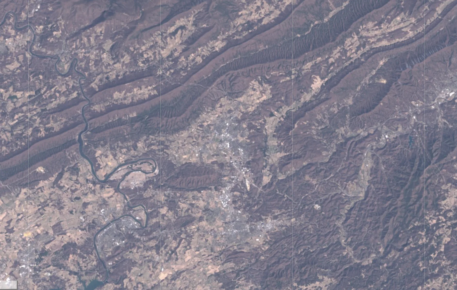
There is more than one way to discover the appropriate min and max values to display. Try going to the Inspector tab and clicking somewhere on the map. The value in each band, in the pixel where you clicked, is displayed as a list in the console. Try clicking on dark and bright objects to get a sense of the range of pixel values. Also, the Earth Engine Code Editor guide describes the layer manager in the upper right of the map display, which lets you automatically compute a linear stretch based on the pixels in the map display.

2.3.2 - False Color Composite

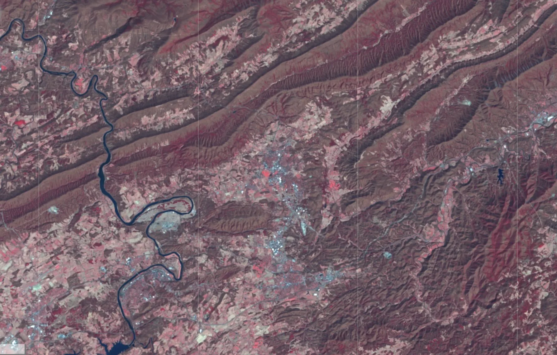
Let’s do the same thing, but this time we will build a false-color composite. This particular set of bands results in a color-IR composite because the near infra-red (NIR) band is set to red. As you inspect the map, look at the pixel values and try to find relationships between the NIR band and different land types. Using false color composites is a very common and powerful method of identifying land characteristics by leveraging the power of signals outside of the visible realm. Mining engineers commonly use hyperspectral data to pinpoint composites with unique signatures, and urban growth researchers commonly use the infrared band to pinpoint roads and urban areas.

// Code Chunk 03
var lat = 37.22; var lon = -80.42;
var zoom = 11;
var image_collection_name = "LANDSAT/LC08/C02/T1";
var date_start = '2014-01-01';
var date_end = '2014-12-31';

var point = ee.Geometry.Point([lon, lat]);
var landsat = ee.ImageCollection(image_collection_name);
//  Note that we need to cast the result of first() to Image.
var image = ee.Image(landsat
                     //  Filter to get only images in the specified range.
                     .filterDate(date_start, date_end)
                     //  Filter to get only images at the location of the point.
                     .filterBounds(point)
                     //  Sort the collection by a metadata property.
                     .sort('CLOUD_COVER')
                     //  Get the first image out of this collection.
                     .first());
//  Print the information to the console
print('A Landsat scene:', image);
//  Define false-color visualization parameters.
var falseColor = {
  bands: ['B5', 'B4', 'B3'],
  min: 4000,
  max: 13000
};
// Add the image to the  map, using the visualization parameters.
Map.setCenter(lon, lat, zoom);
Map.addLayer(image, falseColor, 'false-color composite');

# Code Chunk 03
lat = 37.22; lon = -80.42
zoom = 11
image_collection_name = "LANDSAT/LC08/C02/T1"
date_start = '2014-01-01'
date_end = '2014-12-31'
name = 'false-color composite'
point = ee.Geometry.Point([lon, lat])

image = (
    ee.ImageCollection(image_collection_name)
         .filterBounds(point)
         .filterDate(date_start, date_end)
         .sort('CLOUD_COVER')
         .first()
)
print('A Landsat scene:', image.getInfo())

falseColor = {
    'bands': ['B5', 'B4', 'B3'],
    'min': 4000,
    'max': 13000
}

map2 = build_map(lat, lon, zoom, falseColor, image, name)
map2

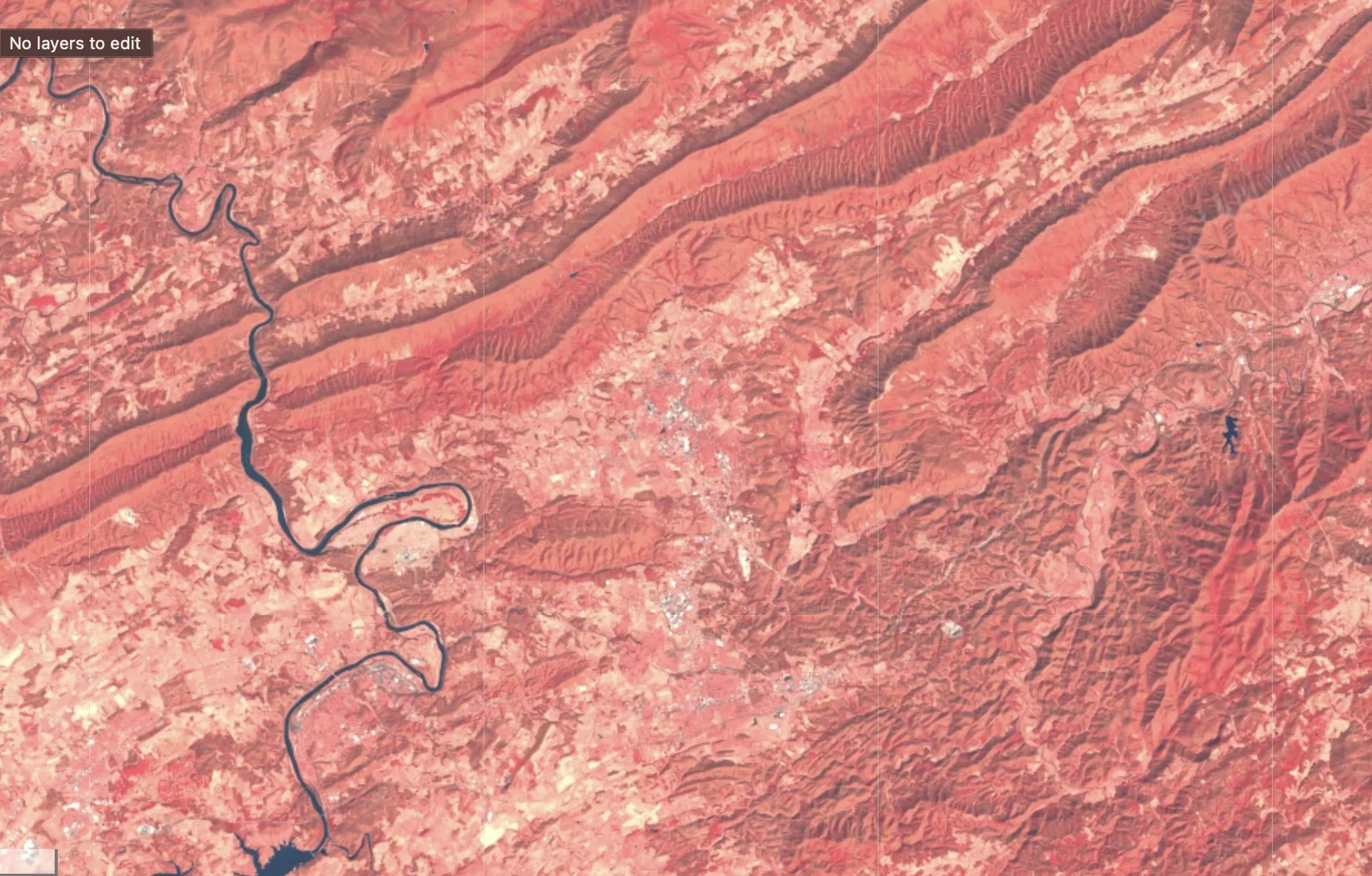
Read through the Landsat data documentation and try playing with different band combinations, min and max values to build different visualizations.

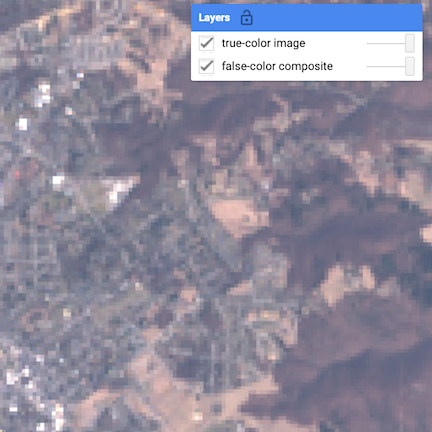
Unique Feature: You can include multiple visualization parameters in your script and toggle the layers on and off with the layer manager for easy comparison.

2.4 - At-Sensor Radiance

The image data you have used so far is stored as a digital number that measures the intensity within the bit range - if data is collected in an 8-bit system, 255 would be very high intensity and 0 will be no intensity. To convert each digital number into a physical unit (at-sensor radiance in Watts/m2/sr/𝝁m), we can use a linear equation:

$$ L_{\lambda} = a_{\lambda} * DN_{\lambda} + b_{\lambda} \qquad $$

Note that every term is indexed by lambda ($\lambda$, the symbol for wavelength) because the coefficients are different in each band. See Chander et al. (2009) for details on this linear transformation between DN and radiance. In this exercise, you will generate a radiance image and examine the differences in radiance from different targets.

Earth Engine provides built-in functions for converting Landsat imagery to radiance in Watts/m2/sr/𝝁m. It will automatically reference the metadata values for each band and apply the equation for you, saving you the trouble of conducting numerous calculations.

This code applies the transformation to a subset of bands (specified by a list of band names) obtained from the image using select(). That is to facilitate interpretation of the radiance spectrum by removing the panchromatic band (‘B8’), an atmospheric absorption band (‘B9’) and the QA bands (‘QA_PIXEL’ and ‘QA_RADSAT’).

Note that the visualization parameters are different to account for the radiance units.

// Code Chunk 4
var lat = 37.22; var lon = -80.42;
var zoom = 11;
var date_start = '2014-01-01';
var date_end = '2014-12-31';
var point = ee.Geometry.Point([lon, lat]);
var landsat = ee.ImageCollection("LANDSAT/LC08/C02/T1");
//  Note that we need to cast the result of first() to Image.
var image = ee.Image(landsat
                     //  Filter to get only images in the specified range.
                     .filterDate(date_start, date_end)
                     //  Filter to get only images at the location of the point.
                     .filterBounds(point)
                     //  Sort the collection by a metadata property.
                     .sort('CLOUD_COVER')
                     //  Get the first image out of this collection.
                     .first());
//  Use these bands.
var bands = ['B1', 'B2', 'B3', 'B4', 'B5', 'B6', 'B7', 'B10', 'B11'];
// Get an image that  contains only the bands of interest.
var dnImage = image.select(bands);
// Apply the  transformation.
var radiance =  ee.Algorithms.Landsat.calibratedRadiance(dnImage);
// Display the result.
var radParams = {bands: ['B5', 'B4', 'B3'], min: 20, max: 110};
Map.setCenter(lon, lat, zoom);
Map.addLayer(radiance, radParams, 'radiance');

# Code Chunk 4
lat = 37.22; lon = -80.42
zoom = 11
image_collection_name = "LANDSAT/LC08/C02/T1"
date_start = '2014-01-01'
date_end = '2014-12-31'
name = 'radiance'
point = ee.Geometry.Point([lon, lat])
image = (
    ee.ImageCollection(image_collection_name)
         .filterBounds(point)
         .filterDate(date_start, date_end)
         .sort('CLOUD_COVER')
         .first()
)
bands = ['B1', 'B2', 'B3', 'B4', 'B5', 'B6', 'B7', 'B10', 'B11']
dnImage = image.select(bands)
radiance = ee.Algorithms.Landsat.calibratedRadiance(dnImage)
radParams = {
    'bands': ['B5', 'B4', 'B3'],
    'min': 20,
    'max': 110
}
map3 = build_map(lat, lon, zoom, radParams, radiance, name)
map3

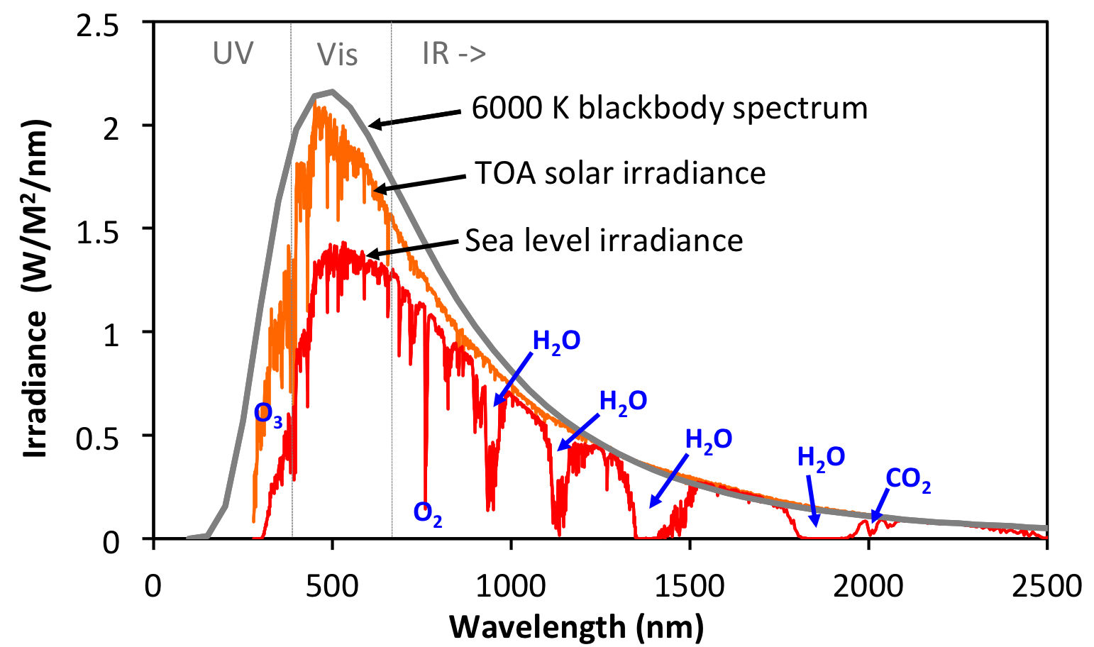
Examine the radiance image by using Inspector and clicking different land cover types on the map near Blacksburg, VA. Click the chart icon in the console to get a bar chart of the different radiance values for each pixel. If the shape of the chart resembles the solar irradiance chart below, that’s because the radiance (in bands 1-7) is mostly reflected solar irradiance. The radiance detected in bands 10-11 is thermal, and is emitted (not reflected) from the surface.

2.5 - Top-of-Atmosphere (TOA) Reflectance

The Landsat sensor is in orbit approximately 700 kilometers above Earth. If we are focused on the imagery of remote sensing (as opposed to studying something like atmospheric conditions or ambient temperature), then we want to find insights about the surface of the earth. To understand the way we calculate information, there are three main components.

Digital Number (DN) is a value that is associated with each pixel - it is generic (in that it is an intensity value dependent upon the bit range), and it allows you to visualize the image where all pixels are in context. DNs are specific to the sensor and the scene, so they are not directly comparable between images; quantitative analysis, machine learning and multi-date work should generally use reflectance instead.

Radiance is the radiation that collected by a sensor - this includes radiation from the surface of Earth, radiation scattered by clouds, position of the sun relative to the Earth and sensor, etc. In general, we want to correct radiance values and convert to reflectance.

Reflectance is the ratio (unitless) of the energy reflected off Earth’s surface to the energy arriving from the sun. In fact, it’s more complicated than this because radiance is a directional quantity, but this definition captures the basic idea. We can identify materials based on their reflectance spectra. Because this ratio is computed using whatever radiance the sensor measures (which may contain all sorts of atmospheric effects), it’s called at-sensor or top-of-atmosphere (TOA) reflectance.

Top of Atmosphere reflectance is the reflectance that includes the radiation from earth’s surface and radiation from earth’s atmosphere.

Let’s examine the spectra for TOA Landsat data. Earth Engine provides Landsat data with the TOA transformation already applied, so we will be using the ‘USGS Landsat 8 Collection 2 Tier 1 TOA Reflectance’ ImageCollection.

// Code Chunk 5
var lat = 37.22; var lon = -80.42;
var zoom = 11;
var date_start = '2014-01-01';
var date_end = '2014-12-31';

var point = ee.Geometry.Point([lon, lat]);
var landsat = ee.ImageCollection("LANDSAT/LC08/C02/T1_TOA");
//  Note that we need to cast the result of first() to Image.
var image = ee.Image(landsat
                     //  Filter to get only images in the specified range.
                     .filterDate(date_start, date_end)
                     //  Filter to get only images at the location of the point.
                     .filterBounds(point)
                     //  Sort the collection by a metadata property.
                     .sort('CLOUD_COVER')
                     //  Get the first image out of this collection.
                     .first());

//  Use these bands.
var bands = ['B1', 'B2', 'B3', 'B4', 'B5', 'B6', 'B7', 'B10', 'B11'];
// Define reflective  bands as bands B1-B7. See the docs for slice().
var reflectiveBands = bands.slice(0, 7);
// See https://www.usgs.gov/faqs/what-are-band-designations-landsat-satellites
var wavelengths = [0.44, 0.48, 0.56, 0.65, 0.86, 1.61, 2.2];
// Select only the  reflectance bands of interest.
var reflectanceImage = image.select(reflectiveBands);

Map.setCenter(lon, lat, zoom);
Map.addLayer(reflectanceImage,
             {bands: ['B4', 'B3', 'B2'],
              min: 0, max: 0.3}, 'toa');
// Define an object of customization parameters for the chart.
var options = {
  title: 'Landsat  8 TOA spectrum in Blacksburg, VA',
               hAxis: {title: 'Wavelength  (micrometers)'},
               vAxis: {title: 'Reflectance'},
               lineWidth: 1,
               pointSize: 4};
// Make the chart, using  a 30 meter pixel.
var chart = ui.Chart.image.regions(
  reflectanceImage,
  point, null, 30, null, wavelengths)
        .setOptions(options);
// Display the chart.
print(chart);

# Code Chunk 5
import matplotlib.pyplot as plt

lat = 37.22; lon = -80.42
zoom = 11
image_collection_name = "LANDSAT/LC08/C02/T1_TOA"
date_start = '2014-01-01'
date_end = '2014-12-31'
name = 'toa'
point = ee.Geometry.Point([lon, lat])

image = (
    ee.ImageCollection(image_collection_name)
         .filterBounds(point)
         .filterDate(date_start, date_end)
         .sort('CLOUD_COVER')
         .first()
)
bands = ['B1', 'B2', 'B3', 'B4', 'B5', 'B6', 'B7', 'B10', 'B11']
# Define reflective bands as bands B1-B7.
reflectiveBands = bands[0:7]
# See https://www.usgs.gov/faqs/what-are-band-designations-landsat-satellites
wavelengths = [0.44, 0.48, 0.56, 0.65, 0.86, 1.61, 2.2]
reflectanceImage = image.select(reflectiveBands)

vizParams = {
    'bands': ['B4', 'B3', 'B2'],
    'min': 0,
    'max': 0.3
}
map4 = build_map(lat, lon, zoom, vizParams, reflectanceImage, name)
display(map4)

# Chart the mean reflectance at the point, using a 30 meter pixel.
vals = reflectanceImage.reduceRegion(ee.Reducer.mean(), point, 30).getInfo()
plt.plot(wavelengths, [vals[b] for b in reflectiveBands], 'o-')
plt.title('Landsat 8 TOA spectrum in Blacksburg, VA')
plt.xlabel('Wavelength (micrometers)')
plt.ylabel('Reflectance')
plt.show()

Since reflectance is a unitless ratio in [0, 1], the visualization parameters above use a min of 0 and a max of 0.3 to display the TOA data.

Using Inspector, click several locations on the map and examine the resultant spectra. If you add the full TOA image (all bands, not only reflectiveBands) as a layer, it becomes apparent that the scale of pixel values in different bands is drastically different. Specifically, bands 10-11 are not in [0, 1]. The reason is that these are thermal bands, and are converted to brightness temperature, in Kelvin, as part of the TOA conversion. Very little radiance is reflected in this wavelength range; most is emitted from the Earth’s surface. That emitted radiance can be used to estimate brightness temperature using the inverted Planck equation. Examine the temperature of various locations. To make plots of reflectance, select the reflective bands from the TOA image and use the Earth Engine charting API.

There are several new methods in this code. The slice() method gets entries in a list based on starting and ending indices. Search the docs (on the Docs tab) for ‘slice’ to find other places this method can be used. Construction of the chart is handled by an object of customization parameters (learn more about customizing charts) passed to ui.Chart.image.regions(). Customizing charts within GEE can be difficult, so spend time modifying the characteristics. In the Python tab, the same values are read with reduceRegion() and plotted with matplotlib.

Question 1: Produce the TOA reflectance plot for Blacksburg, VA and briefly describe the relationship of reflectance peaks and troughs in the chart to the electromagnetic spectrum.

2.6 - Surface Reflectance

The ratio of upward radiance at the Earth’s surface to downward radiance at the Earth’s surface is called surface reflectance. TOA reflectance is computed from the radiance measured at the sensor, so it still includes the effects of the atmosphere: both the inbound and outbound radiance from the sun is affected by its path through the atmosphere to the sensor. Surface reflectance estimates the reflectance at the ground after those atmospheric effects have been removed. Unravelling those effects is called atmospheric correction (“compensation” is probably a more accurate term) and is beyond our scope of this lab. However, most satellite imagery providers complete this correction for the consumers. While you could use the raw scenes directly, if your goal is conduct analysis quickly and effectively, using the corrected Surface Reflectance image collections are quite beneficial and will save you quite a bit of time.

In the datasets page for Landsat 8, it’s broken up into the raw images, TOA, and Surface Reflectance.

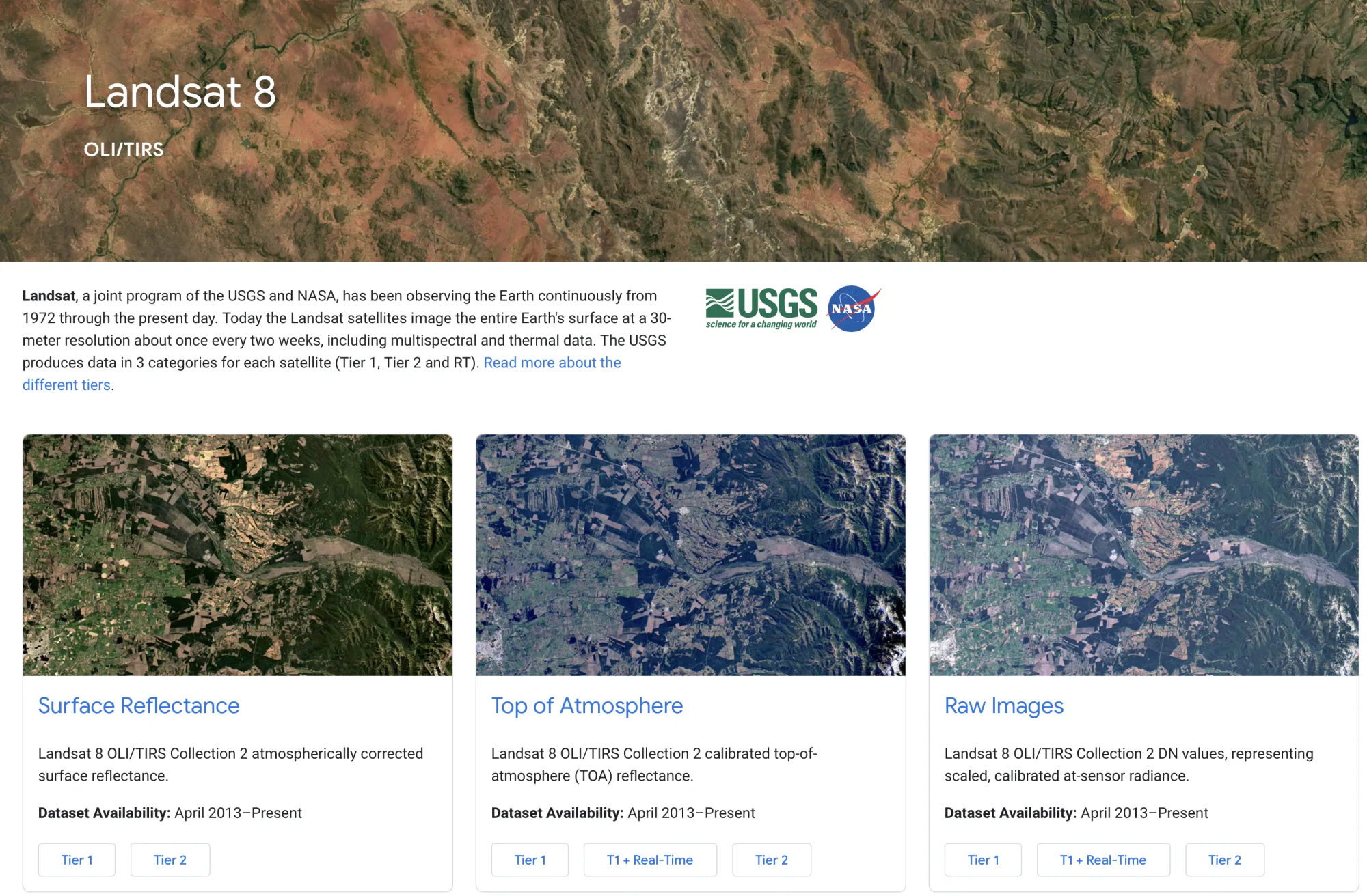
Question 2: Use the code chunk 5 pattern above to build a true-color (red-green-blue) image using Surface Reflectance data from Landsat 8 and a plot with the same wavelengths and structure as you did with the TOA. Produce the surface reflectance plot and briefly describe its features. What differs or remains the same between the TOA plot and the surface reflectance plot?

Note that the band names differ between the surface reflectance data and the TOA data.

Question 3: When you build the surface reflectance visualization, you will need to scale the imagery and change the visualization parameters. Why? Read the dataset description to find out.

Hint: What is the scale factor for the SR_B1 to SR_B7 bands?

Additional Exercises

Question 4: In your code, set the value of a variable called azimuth to the solar azimuth of the image from code chunk 4. Do not hardcode the number. Use get(). Print the result and show you set the value of azimuth.

Question 5: Add a layer to the map in which the image from code chunk 4 is displayed with band 7 set to red, band 5 set to green and band 3 set to blue. Produce the layer and describe how you would display the layer name as falsecolor.

Question 6: What is the brightness temperature of the given Blacksburg, VA point?

Show how you make a variable in your code called temperature and set it to the band 10 brightness temperature. Use this guide for help.

// `image` is the TOA image from code chunk 5.
var point = ee.Geometry.Point([-80.42, 37.22]);

var temperature = image.reduceRegion({
  // YOUR SOLUTION HERE: reducer, geometry and scale
}).get('YOUR_BAND_NAME_HERE');

Question 7: If you plot the Surface Reflectance data with the TOA visibility parameters, you’ll notice that you get a blank image. To fix this issue, we have to apply a scale factor and offset, which can be found in the documentation - note that all the optical bands (SR_B1-SR_B7) share one scale and offset, while the other bands (that start with ST) vary.

Bring in the Landsat Surface Reflectance collection (LANDSAT/LC08/C02/T1_L2), filter it down to one specific image from the point listed above (Blacksburg, VA), and use the multiply and add methods to apply the scale and offset to the optical bands (the Landsat SR code snippet in the catalog shows how).

Then, use the reduceRegion() method to find the reflectance value for band 5. Create a variable named reflectance to store this value and print it to the console. The value should fall into the range of [0-1]